Tutorial: Turning on The Lights
An Introduction to VIIRS Nighttime Imagery
The most familiar views of Earth from space feature a blue-green planet lit by the Sun.
But in the darkness of night when the Moon, city lights, fires, or aurorae illuminate Earth, some satellites continue to gather images of light. And they are fantastic!
So how does such imagery come to be? Let’s take a look!
On my bucket list: seeing the #NorthernLights' brilliant glow overhead.
— Joshua Stevens (@jscarto) March 29, 2019
Until then, Suomi VIIRS provides a spectacular view of auroras from above - like this one on March 28: https://t.co/0RDgyVF20u #AuroraBorealis pic.twitter.com/eZD0VjhrOn
Twice a day, the Suomi NPP and NOAA-20 satellites capture a global view of Earth—once during day, once at night. Both satellites are equipped with a Visible Infrared Imaging Radiometer Suite (VIIRS) instrument. Among the capabilities of VIIRS is the “day/night band,” or DNB. The highly sensitive DNB collects measurements of light from below, with adjustments to ensure each pixel acquired is neither overly bright or too dark.
When it comes to DNB, VIIRS is poetically sensitive. So much so that the instrument is able to detect startlight from our galaxy as it scatters across Earth’s atmosphere. (I am imagining here scenes described in The Silmarillion, as Tolkien’s elves stare longingly skyward at the faint glow of many stars.)
VIIRS really is incredible. Let’s take a look at the process of acquiring DNB data and producing imagery.
This tutorial requires GDAL and some basic familiarity with the command line.
Acquiring Data
We’ll be using the Level-1B DNB data from Suomi, known as “NPP_VDNES_L1.” The Suomi VIIRS DNB data have a spatial resolution of 750 m/px and are available from January 19, 2012—present.
Go to the LAADS DAAC data portal.
The link above will automatically select the NPP_VDNES_L1 product for you. Ensure to select it otherwise.
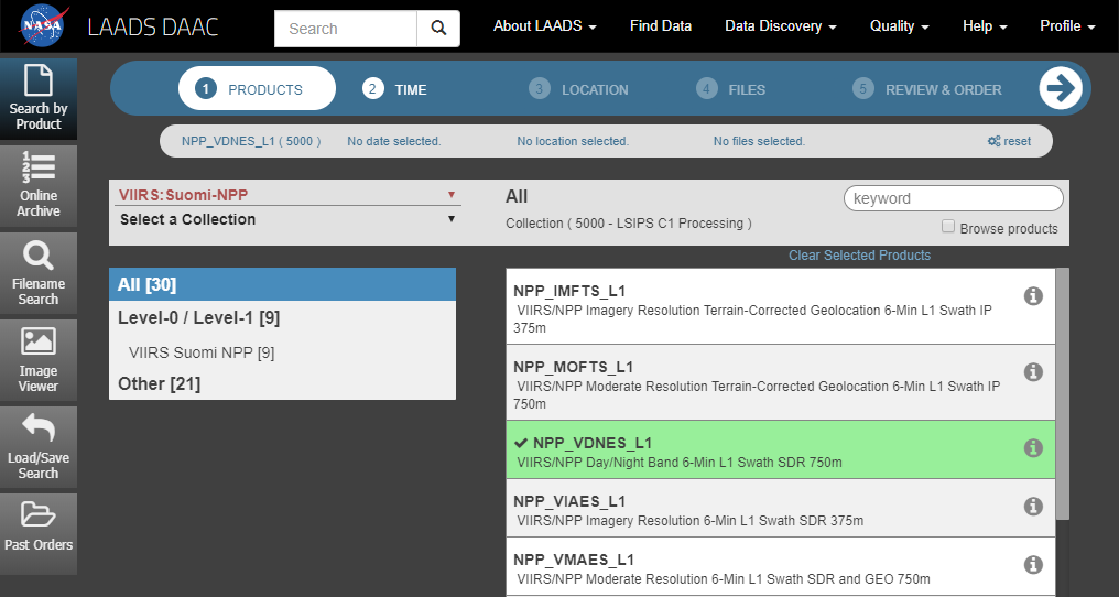
With the correct data selected, we must now chose a time (or time period) in which to search for files.
Click Time at the top of the data portal, select Single Date, and then enter date of interest. For the coverage selection, uncheck Day, then check the boxes for Night and Day-Night Boundary.
I’ve chosen March 26, 2019, which offered a clear view of the Great Lakes.
Click Add Date.

The correct data is chosen. A time has been selected. Now we just need to subset the search by location.
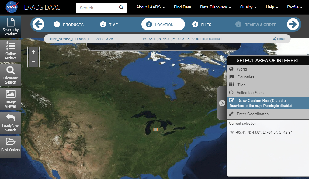
Click Location at the top of the data portal. You will be presented with a map view.
From here, you can choose a location in a variety of ways. Since I want to see the Great Lakes, I’ve zoomed and panned the map to the general area.
I then used the Draw Custom Box tool to draw a box that falls within the area I want to download.
 Note: The search will find all data granules that intersect the drawn box. It will not crop the data to the box!
Click Files at the top of the data portal. This will return a list of files that match your criteria.

Since VIIRS Level-1 granules are quite wide, there is a good chance you will receive several results for a given location. One or more of these results will contain your location well within the granule, while others might barely overlap at the edge of the granule. VIIRS data is noisier at the edges, so you want the granule(s) that contain your location as close to the center as possible.
Knowing which file(s) to download takes a bit of investigation. The nighttime orbit of Suomi can be viewed in Worldview, which shows the times (in UTC) and location of the satellite. Change the date and move the map around to see the oribital path specific to the time and place you’re interested in.
The orbit of Suomi on March 26 shows that VIIRS got two views of the Great Lakes, once at about 6:50 and again around 8:40 UTC.
A more centered view comes from the orbit that happened around 6:50, so that’s what I want to look for in the search results.
The first file in the results from the data portal was acquired at 2019-03-26 06:54:00. That’s the one I want!
In the NASA Earthdata portal, click the download icon next to your file of choice to begin downloading the data. The data will be an HDF file.
With the data handy, it is time to process it into imagery.
Producing Imagery
Being an HDF (Hierarchical Data Format), the DNB data includes multiple variables, arranged in a well-defined structure.
GDAL makes it easy to look at this structure and find the variable(s) from which imagery can be produced.
For instance, if you had a file named MY_FILE, the command gdalinfo MY_FILE will output information about that file, including its data and subdatasets, dimensions, spatial projection, and other metadata.
Go ahead and try it on the DNB data file. You will see a lot of information.
We want to get the full path to the DNB data for mapping. The variable within this file that we’ll be using is called Radiance. (The units are watts per square centimeter per steradian, W cm-2 sr-1.)
The full HDF path to the Radiance variable can be retried via:
gdalinfo NPP_VDNES_L1.A2019085.0654.001.2019085123230.hdf | grep Radiance
In the output, one line includes NAME=, followed by the full path to the variable. For the file I’ve downloaded, this is:
HDF4_EOS:EOS_SWATH:"NPP_VDNES_L1.A2019085.0654.001.2019085123230.hdf":VIIRS_EV_DNB_SDR:Radiance
Note that this is just the filename in quotations, with HDF4_EOS:EOS_SWATH: prepended to the front, and :VIIRS_EV_DNB_SDR:Radiance appended to the end. These tell GDAL which kind of file it is working with (HDF has many varieties), the name of the file, and where to find the data within the file.
Initial Geolocation and Reprojection
The first thing to do is reproject the data and output the variable of interest to a simpler GeoTIFF.
Using the full path to the Radiance variable, we can now use gdalwarp to:
- Reproject the variable
- Ensure the resolution remains 750 m/px
- Define a resampling method used during the reprojection
- Geolocate the variable from geolocation arrays within the data
- Output a GeoTIFF
This all happens in the command below, which reprojects the data from WGS84 to EPSG:5070 (CONUS Albers Equal Area).
gdalwarp -s_srs WGS84 -t_srs EPSG:5070\
    -tr 750 750\
    -r bilinear\
    -geoloc\
    'HDF4_EOS:EOS_SWATH:"NPP_VDNES_L1.A2019085.0654.001.2019085123230.hdf":VIIRS_EV_DNB_SDR:Radiance'\
    greatlakes_vir_dnb.tif
The resulting GeoTIFF (greatlakes_vir_dnb.tif) would work well in almost any GIS software, though it will need to be “stretched” between some minimum and maximum value. But if you tried to open it in Photoshop or other image programs, it will probably look like a whole lot of nothing.
This is because the units for DNB Radiance are incredibly small, and the data are 32-bit floating point numbers. Most photo software is not designed for this precision.
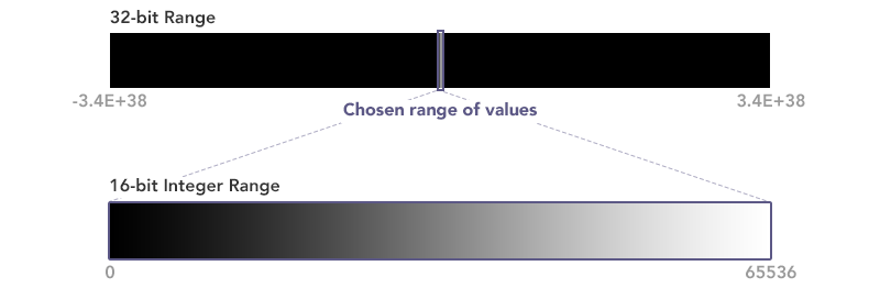
We can solve that by converting the data to 16-bit integers, scaled to a smaller range of values.
Scaling the data
Rather than asking photo software or web browsers to display the full 32-bit range, which would result in an almost entirely black image, we can scale a small portion of the radiance–where visible data actually exists–across the smaller integer range. This “stretching” will make the data immediately visible.
Stretching can be accomplished with gdal_translate. To produce a visible image, a few things should be done:
- Convert the data to 16-bit unsigned integers
- Data values [0 - 0.000000008] stretched to [0 - 65536]
- Resize the image to 800px wide (for display online) using bilinear resampling
The command below does that:
gdal_translate -ot UInt16 -scale 0 8e-9 0 65536\
    -outsize 800 0 -r bilinear\
    greatlakes_vir_dnb.tif greatlakes_vir_dnb_int.tif
Excellent! We now have a visible image of the data.

City lights around the Great Lakes shine brightly under the relatively clear skies of March 26, 2019. The GeoTIFF was saved as a JPEG for smaller size on the web.
There is nothing special about the value 0.000000008 (8e-9). It is just a temporary starting point to produce a visible image.
In the image above, city lights, some of the landscape, and clouds over the Atlantic are easily visible. The brightest parts of the cities are a bit too bright—our stretch needs some fine tuning. Each image will have its own assortment of values, and features within the image, that require some tweaking.
One might even apply a logarithmic or square root stretch, which can help emphasize dimmer lights without overblowing clouds or super bright areas. I used a square root stretch when creating the 2016 and 2012 Black Marble imagery.
Some outlets automate this processing with a consistent stretch. This works well for getting an overall sense of the data, but is not optimal. An image of city lights will need to be stretched differently from one that emphasizes an aurora, for instance.
But you are now equipped to start making these decisions to process the data in a way that fits your needs and end results!
Notes and Caveats
Nightlights imagery has been particularly desirable for newsrooms. With countries experiencing power outages, due to manmade or natural causes, showing a before-and-after comparison is appealing.
Pump the brakes! Recall that VIIRS DNB is mind-blowingly sensitive. The overall brightness or dimness of an area is not without influence from moonlight (and the phase of the moon), the albedo of the landscape—including snow or other seasonal variations, airglow, and even distant stars! It is easy to be misled. A thin veil of clouds can make dim city lights appear larger and brighter, as the light is spread around more diffusely. All of this needs to be accounted for to ensure the changes you see are actually changes in the lighting conditions of interest, and not changes in the environmental conditions.
Techniques that normalize the data for these factors exist. Most commonly this is through a Bidirectional Reflectance Distribution Function (BRDF). For VIIRS DNB data, this is not straightforward and requires the collection of daytime DNB imagery to determine parameters used in the analysis, among other considerations.
NASA scientists are producing a version of VIIRS DNB data with atmospheric and BRDF corrections. For analytical purposes, this type of data should be preferred. In any case, it is best to speak to a scientist before drawing conclusions from changes observed in DNB imagery.
This is primarily a concern for comparative analysis. For viewing features at a single point in time (auroras, wildfires, sea ice, and so on), the processing shown here will get you off to a great start.
So turn on the lights and start making some nighttime images! If you do produce some imagery I would love to see it.
Links and Further Reading
Earth at Night imagery from NASA Earth Observatory
Nightly preview of VIIRS DNB data in NASA Worldview
Curtis Seaman, CIRA/Colorado State University. Beginner’s Guide to VIIRS Imagery Data [PDF]
Román, Miguel O., et al. (2018). NASA’s Black Marble Nighttime Lights Product Suite. Remote Sensing of Environment, 210, 113-143.
Straka, W. et al. (2015). Using VIIRS DNB to Detect Natural (and other) Disasters [PDF]